Dipl.-Ing. Julia Schachtschneider
Erstbetreuer: C. Brenner; Co-Betreuer: M. Sester
In the context of autonomous driving, there is a strong demand for high precision and up-to-date models of the environment. As natural environments are constantly changing, one of the biggest challenges is to identify and model these changes. There are static objects, which are unlikely to change, like building façades, and there are dynamic objects, like vegetation, which changes with different seasons, or parked cars, which change their position in a daily or weekly cycle. A frequent solution is to remove all non-static parts of the environment from the map. This has the disadvantage that a large amount of possibly useful information is also discarded.
In this project, we work on the development of an environment model that includes temporal effects. As a result, we want to provide a map that represents the dynamic processes of an urban environment and contains a probabilistic description of all objects at any point in time.
If a robotic system like a self-driving car only uses a static map, all measurements of changing objects would cause conflicts with the map. Furthermore, areas with only few static components could have a very poor map. Since our model includes such temporal effects, changes are “expected” by the robot. Furthermore, in areas with only few static objects, the map still contains the changeable parts of the environment and even if those have a lower accuracy, a coarse localization is still possible.
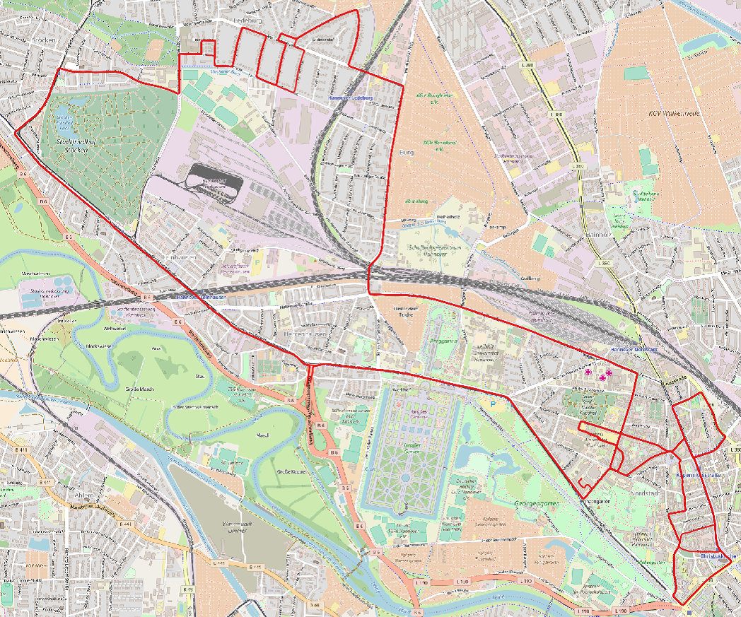
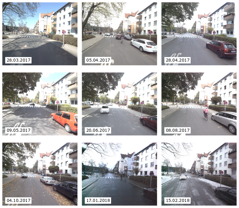
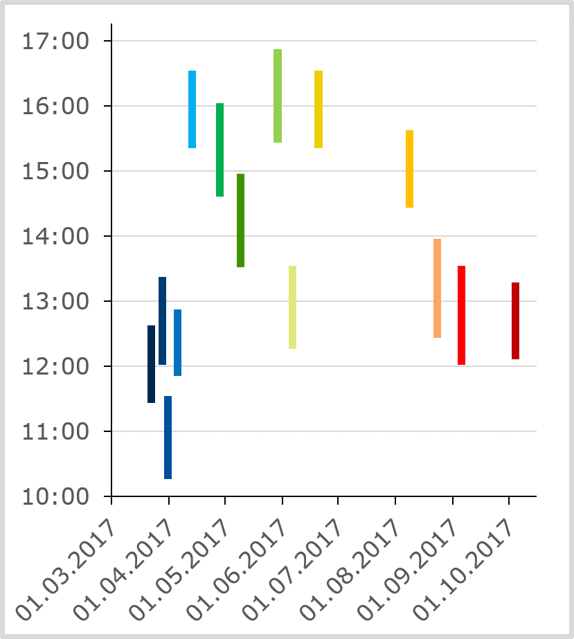
For this project, we have recorded an extensive long-term data set. Therefore, we carried out measurement campaigns with a LiDAR Mobile Mapping System about every two weeks (from March 2017 until March 2018). We have chosen a route in Hannover, Germany, with an approximate length of 20 km (see fig. 2). The measurement area partly overlaps with the area of the i.c.sens mapathons and covers inner city areas as well as residential districts, different kinds of roads (one-way, multi-lane and shared with tramlines), various intersections, parking lots, areas with high pedestrian and/ or bicycle traffic. The resulting data set includes all different seasons (from leafless vegetation through growing season, etc.) as well as different weather and lighting conditions (sunny, overcast sky, twilight, darkness, and snow-covered roads). Fig. 3 shows an example of the different measurement conditions.
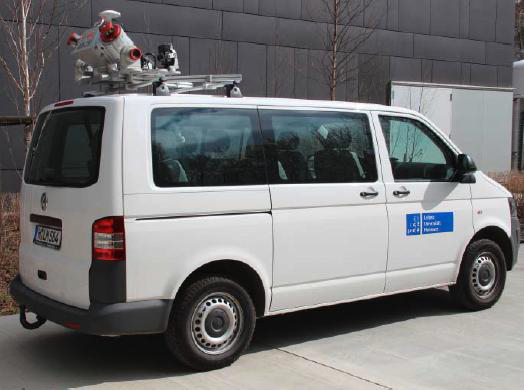
For data acquisition, we used a Riegl-VMX Mobile Mapping System (MMS), mounted on a measurement vehicle as shown in fig. 1. The MMS is equipped with two Riegl VQ-250 laser scanners and four cameras. For localization, it uses a highly accurate GNNS/IMU System, combined with a Distance Measurement Instrument (DMI). Aside from direct georeferencing, a least squares adjustment is used to obtain a very high precision alignment of all measurement campaigns, resulting in aligned point clouds with billions of points.
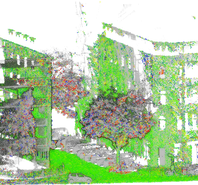
This project uses mainly post-processed and aligned LiDAR point clouds. Fig. 4 shows an example point cloud, containing measurements from 14 campaigns.
For our environment model, we decided to use a voxel grid representation of the environment. As the aligned point clouds usually have a standard deviation below two centimeters, the grid cells can be very small. We insert the LiDAR points into our voxel grid. Using a full ray tracing, we are able to identify not only the cells which contain a measured point, but also cells which are traversed by a ray and thus can be considered being unoccupied. Consequently, each voxel stores an observation sequence with one state for each measurement run. The state can be ether “occupied” (contains a reflecting point for this measurement), “free” (no reflecting point and traversed by a laser ray) or “unknown” (no information). This occupancy grid is the basis for our map.
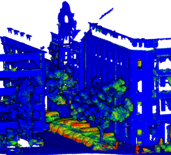
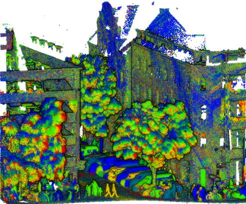
As a first and simple solution for a reference map (baseline) we introduced a confidence score for each voxel (number of free/ number of occupied states in one sequence), which is a measure whether the voxel is part of a static object or more temporary/ dynamic. Fig. 5 shows an example point cloud colored by the confidence score.
This baseline approach has the before mentioned disadvantage that although it includes dynamic objects, their behavior is not modelled. The likelihood of a measurement consists of two components: “Is the measured object present?” (voxel occupied) and “Is the object visible?” (in the measurement area and not occluded). These two criterions strongly depend on the object class of the measured points. For example, a façade behind a tree is always present, but in summer, it is very likely to be occluded by the foliage of the tree in front of it (see the blue areas on the right façade in fig. 4).
In order to take into account these two factors, we decided to use a beam model, which models the interaction of the laser ray with the environment. We have demonstrated that for localization, a map from the same season works best. Fig. 6 shows the example area with a voxel map (grey) from a measurement run at the beginning of June compared to a point cloud from a test run at the end of June. On the façades, the measured points mostly lie inside the corresponding voxels. Points on vegetation and parked cars had a larger distance to the closest voxel in the map or there was no corresponding voxel found.
The localization result can be further improved if the map is composed of more measurement runs. However, the more information the map contains, the more "weak" correspondences are found. At some point the positive effect is reversed, a lot of poor correlations are included in the result and the localization deteriorates. We are currently developing a measurement model, which contains a weighting of the corresponding voxels along the ray in dependence of the object class entered in the map. Therefore, we use classification results from project 3 (semantic segmentation) and investigate the individual temporal behavior of the object classes.